Introduction

Data Structure can be defined as the group of data elements which provides an efficient way of storing and organising data in the computer so that it can be used efficiently. Some examples of Data Structures are arrays, Linked List, Stack, Queue, etc. Data Structures are widely used in almost every aspect of Computer Science i.e. Operating System, Compiler Design, Artifical intelligence, Graphics and many more.

Data Structures are the main part of many computer science algorithms as they enable the programmers to handle the data in an efficient way. It plays a vitle role in enhancing the performance of a software or a program as the main function of the software is to store and retrieve the user’s data as fast as possible

Basic Terminology

Data structures are the building blocks of any program or the software. Choosing the appropriate data structure for a program is the most difficult task for a programmer. Following terminology is used as far as data structures are concerned

Data: Data can be defined as an elementary value or the collection of values, for example, student’s name and its id are the data about the student.

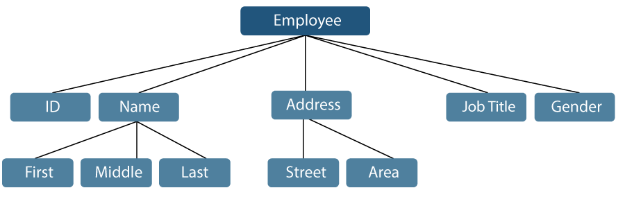
Group Items: Data items which have subordinate data items are called Group item, for example, name of a student can have first name and the last name.

Record: Record can be defined as the collection of various data items, for example, if we talk about the student entity, then its name, address, course and marks can be grouped together to form the record for the student.

File: A File is a collection of various records of one type of entity, for example, if there are 60 employees in the class, then there will be 20 records in the related file where each record contains the data about each employee.

Attribute and Entity: An entity represents the class of certain objects. it contains various attributes. Each attribute represents the particular property of that entity.

Field: Field is a single elementary unit of information representing the attribute of an entity.

Need of Data Structures

As applications are getting complexed and amount of data is increasing day by day, there may arrise the following problems:

Processor speed: To handle very large amout of data, high speed processing is required, but as the data is growing day by day to the billions of files per entity, processor may fail to deal with that much amount of data.

Data Search: Consider an inventory size of 106 items in a store, If our application needs to search for a particular item, it needs to traverse 106 items every time, results in slowing down the search process.

Multiple requests: If thousands of users are searching the data simultaneously on a web server, then there are the chances that a very large server can be failed during that process

in order to solve the above problems, data structures are used. Data is organized to form a data structure in such a way that all items are not required to be searched and required data can be searched instantly.

Advantages of Data Structures

Efficiency: Efficiency of a program depends upon the choice of data structures. For example: suppose, we have some data and we need to perform the search for a perticular record. In that case, if we organize our data in an array, we will have to search sequentially element by element. hence, using array may not be very efficient here. There are better data structures which can make the search process efficient like ordered array, binary search tree or hash tables.

Reusability: Data structures are reusable, i.e. once we have implemented a particular data structure, we can use it at any other place. Implementation of data structures can be compiled into libraries which can be used by different clients.

Abstraction: Data structure is specified by the ADT which provides a level of abstraction. The client program uses the data structure through interface only, without getting into the implementation details.

Data Structure Classification

Linear Data Structures: A data structure is called linear if all of its elements are arranged in the linear order. In linear data structures, the elements are stored in non-hierarchical way where each element has the successors and predecessors except the first and last element.

Types of Linear Data Structures are given below:Arrays: An array is a collection of similar type of data items and each data item is called an element of the array. The data type of the element may be any valid data type like char, int, float or double.

The elements of array share the same variable name but each one carries a different index number known as subscript. The array can be one dimensional, two dimensional or multidimensional.

The individual elements of the array age are:

age[0], age[1], age[2], age[3],……… age[98], age[99].

Linked List: Linked list is a linear data structure which is used to maintain a list in the memory. It can be seen as the collection of nodes stored at non-contiguous memory locations. Each node of the list contains a pointer to its adjacent node.

Stack: Stack is a linear list in which insertion and deletions are allowed only at one end, called top.

A stack is an abstract data type (ADT), can be implemented in most of the programming languages. It is named as stack because it behaves like a real-world stack, for example: – piles of plates or deck of cards etc.

Queue: Queue is a linear list in which elements can be inserted only at one end called rear and deleted only at the other end called front.

It is an abstract data structure, similar to stack. Queue is opened at both end therefore it follows First-In-First-Out (FIFO) methodology for storing the data items.

Non Linear Data Structures: This data structure does not form a sequence i.e. each item or element is connected with two or more other items in a non-linear arrangement. The data elements are not arranged in sequential structure.

Types of Non Linear Data Structures are given below:

Trees: Trees are multilevel data structures with a hierarchical relationship among its elements known as nodes. The bottommost nodes in the herierchy are called leaf node while the topmost node is called root node. Each node contains pointers to point adjacent nodes.

Tree data structure is based on the parent-child relationship among the nodes. Each node in the tree can have more than one children except the leaf nodes whereas each node can have atmost one parent except the root node. Trees can be classfied into many categories which will be discussed later in this tutorial.

Graphs: Graphs can be defined as the pictorial representation of the set of elements (represented by vertices) connected by the links known as edges. A graph is different from tree in the sense that a graph can have cycle while the tree can not have the one.

Operations on data structure

1) Traversing: Every data structure contains the set of data elements. Traversing the data structure means visiting each element of the data structure in order to perform some specific operation like searching or sorting.

Example: If we need to calculate the average of the marks obtained by a student in 6 different subject, we need to traverse the complete array of marks and calculate the total sum, then we will devide that sum by the number of subjects i.e. 6, in order to find the average.

2) Insertion: Insertion can be defined as the process of adding the elements to the data structure at any location.

If the size of data structure is n then we can only insert n-1 data elements into it.

3) Deletion:The process of removing an element from the data structure is called Deletion. We can delete an element from the data structure at any random location.

If we try to delete an element from an empty data structure then underflow occurs.

4) Searching: The process of finding the location of an element within the data structure is called Searching. There are two algorithms to perform searching, Linear Search and Binary Search. We will discuss each one of them later in this tutorial.

5) Sorting: The process of arranging the data structure in a specific order is known as Sorting. There are many algorithms that can be used to perform sorting, for example, insertion sort, selection sort, bubble sort, etc.

6) Merging: When two lists List A and List B of size M and N respectively, of similar type of elements, clubbed or joined to produce the third list, List C of size (M+N), then this process is called merging

Array

Definition

• Arrays are defined as the collection of similar type of data items stored at contiguous memory locations.
• Arrays are the derived data type in C programming language which can store the primitive type of data such as int, char, double, float, etc.
• Array is the simplest data structure where each data element can be randomly accessed by using its index number.
• For example, if we want to store the marks of a student in 6 subjects, then we don’t need to define different variable for the marks in different subject. instead of that, we can define an array which can store the marks in each subject at a the contiguous memory locations.

The array marks[10] defines the marks of the student in 10 different subjects where each subject marks are located at a particular subscript in the array i.e. marks[0] denotes the marks in first subject, marks[1] denotes the marks in 2nd subject and so on.

Properties of the Array

1. Each element is of same data type and carries a same size i.e. int = 4 bytes.
2. Elements of the array are stored at contiguous memory locations where the first element is stored at the smallest memory location.
3. Elements of the array can be randomly accessed since we can calculate the address of each element of the array with the given base address and the size of data element.

for example, in C language, the syntax of declaring an array is like following:

1. int arr[10]; char arr[10]; float arr[5]   

Need of using Array

In computer programming, the most of the cases requires to store the large number of data of similar type. To store such amount of data, we need to define a large number of variables. It would be very difficult to remember names of all the variables while writing the programs. Instead of naming all the variables with a different name, it is better to define an array and store all the elements into it.

Following example illustrates, how array can be useful in writing code for a particular problem.

In the following example, we have marks of a student in six different subjects. The problem intends to calculate the average of all the marks of the student.

In order to illustrate the importance of array, we have created two programs, one is without using array and other involves the use of array to store marks.

Program without array:

1. #include <stdio.h>  
2. void main ()  
3. {  
4.     int marks_1 = 56, marks_2 = 78, marks_3 = 88, marks_4 = 76, marks_5 = 56, marks_6 = 89;   
5.     float avg = (marks_1 + marks_2 + marks_3 + marks_4 + marks_5 +marks_6) / 6 ;   
6.     printf(avg);   
7. }  

Program by using array:

1. #include <stdio.h>  
2. void main ()  
3. {  
4.     int marks[6] = {56,78,88,76,56,89);  
5.     int i;    
6.     float avg;  
7.     for (i=0; i<6; i++ )   
8.     {  
9.         avg = avg + marks[i];   
10.     }    
11.     printf(avg);   
12. }   

Advantages of Array

• Array provides the single name for the group of variables of the same type therefore, it is easy to remember the name of all the elements of an array.
• Traversing an array is a very simple process, we just need to increment the base address of the array in order to visit each element one by one.
• Any element in the array can be directly accessed by using the index.

Memory Allocation of the array

As we have mentioned, all the data elements of an array are stored at contiguous locations in the main memory. The name of the array represents the base address or the address of first element in the main memory. Each element of the array is represented by a proper indexing.

The indexing of the array can be defined in three ways.

1. 0 (zero – based indexing) : The first element of the array will be arr[0].
2. 1 (one – based indexing) : The first element of the array will be arr[1].
3. n (n – based indexing) : The first element of the array can reside at any random index number.

In the following image, we have shown the memory allocation of an array arr of size 5. The array follows 0-based indexing approach. The base address of the array is 100th byte. This will be the address of arr[0]. Here, the size of int is 4 bytes therefore each element will take 4 bytes in the memory.

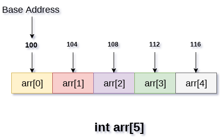
In 0 based indexing, If the size of an array is n then the maximum index number, an element can have is n-1. However, it will be n if we use 1 based indexing.

Accessing Elements of an array

To access any random element of an array we need the following information:

1. Base Address of the array.
2. Size of an element in bytes.
3. Which type of indexing, array follows.

Address of any element of a 1D array can be calculated by using the following formula:

1. Byte address of element A[i]  = base address + size * ( i – first index)   

Example :

1. In an array, A[-10 ….. +2 ], Base address (BA) = 999, size of an element = 2 bytes,   
2. find the location of A[-1].  
3. L(A[-1]) = 999 + [(-1) – (-10)] x 2  
4.        = 999 + 18   
5.        = 1017   

2D Array

2D array can be defined as an array of arrays. The 2D array is organized as matrices which can be represented as the collection of rows and columns.

However, 2D arrays are created to implement a relational database look alike data structure. It provides ease of holding bulk of data at once which can be passed to any number of functions wherever required.

How to declare 2D Array

The syntax of declaring two dimensional array is very much similar to that of a one dimensional array, given as follows.

1. int arr[max_rows][max_columns];   

however, It produces the data structure which looks like following.

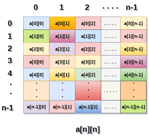
Above image shows the two dimensional array, the elements are organized in the form of rows and columns. First element of the first row is represented by a[0][0] where the number shown in the first index is the number of that row while the number shown in the second index is the number of the column.

How do we access data in a 2D array

Due to the fact that the elements of 2D arrays can be random accessed. Similar to one dimensional arrays, we can access the individual cells in a 2D array by using the indices of the cells. There are two indices attached to a particular cell, one is its row number while the other is its column number.

However, we can store the value stored in any particular cell of a 2D array to some variable x by using the following syntax.

1. int x = a[i][j];   

where i and j is the row and column number of the cell respectively.

We can assign each cell of a 2D array to 0 by using the following code:

1. for ( int i=0; i<n ;i++)  
2. {  
3.     for (int j=0; j<n; j++)   
4.     {  
5.         a[i][j] = 0;   
6.     }  
7. }  

Initializing 2D Arrays

We know that, when we declare and initialize one dimensional array in C programming simultaneously, we don’t need to specify the size of the array. However this will not work with 2D arrays. We will have to define at least the second dimension of the array.

The syntax to declare and initialize the 2D array is given as follows.

1. int arr[2][2] = {0,1,2,3};   

The number of elements that can be present in a 2D array will always be equal to (number of rows * number of columns).

Example : Storing User’s data into a 2D array and printing it.

C Example :

1. #include <stdio.h>  
2. void main ()  
3. {  
4.     int arr[3][3],i,j;   
5.     for (i=0;i<3;i++)  
6.     {  
7.         for (j=0;j<3;j++)  
8.         {  
9.             printf(“Enter a[%d][%d]: “,i,j);              
10.             scanf(“%d”,&arr[i][j]);  
11.         }  
12.     }  
13.     printf(“\n printing the elements ….\n”);   
14.     for(i=0;i<3;i++)  
15.     {  
16.         printf(“\n”);  
17.         for (j=0;j<3;j++)  
18.         {  
19.             printf(“%d\t”,arr[i][j]);  
20.         }  
21.     }  
22. }  

Sparse matrix

A sparse matrix is a one in which the majority of the values are zero. The proportion of zero elements to non-zero elements is referred to as the sparsity of the matrix. The opposite of a sparse matrix, in which the majority of its values are non-zero, is called a dense matrix.

Sparse matrices are used by scientists and engineers when solving partial differential equations. For example, a measurement of a matrix’s sparsity can be useful when developing theories about the connectivity of computer network.When using large sparse matrices in a computer program, it is important to optimize the data structures and algorithm to take advantage of the fact that most of the values will be zero.

Sparse matrix example

Here is an example of a 4 x 4 matrix containing 12 zero values and 4 non-zero values, giving it a sparsity of 3:

[[5, 0, 0, 0],
[0, 11, 0, 0],
[0, 0, 25, 0],
[0, 0, 0, 7]]

Representing a sparse matrix by a 2D array leads to wastage of lots of memory as zeroes in the matrix are of no use in most of the cases. So, instead of storing zeroes with non-zero elements, we only store non-zero elements. This means storing non-zero elements with triples- (Row, Column, value).

Sparse Matrix Representations can be done in many ways following are two common representations:

1. Array representation
2. Linked list representation

Method 1: Using Arrays

2D array is used to represent a sparse matrix in which there are three rows named as

• Row: Index of row, where non-zero element is located
• Column: Index of column, where non-zero element is located
• Value: Value of the non zero element located at index – (row,column)

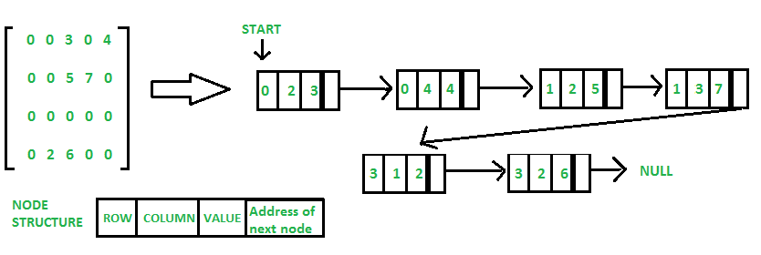
Method 2: Using Linked Lists

In linked list, each node has four fields. These four fields are defined as:

• Row: Index of row, where non-zero element is located
• Column: Index of column, where non-zero element is located
• Value: Value of the non zero element located at index – (row,column)
• Next node: Address of the next node

• Upper and Lower Triangular Matrices:
– Definition: An upper triangular matrix is a square matrix in which all entries below the main
diagonal are zero (only nonzero entries are found above the main diagonal – in the upper triangle).
A lower triangular matrix is a square matrix in which all entries above the main diagonal are zero
(only nonzero entries are found below the main diagonal – in the lower triangle). See the picture
below.
– Notation: An upper triangular matrix is typically denoted with U and a lower triangular matrix
is typically denoted with L.
– Properties: