Process

A process is basically a program in execution. The execution of a process must progress in a sequential fashion.

A process is defined as an entity which represents the basic unit of work to be implemented in the system.

To put it in simple terms, we write our computer programs in a text file and when we execute this program, it becomes a process which performs all the tasks mentioned in the program.

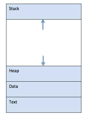
When a program is loaded into the memory and it becomes a process, it can be divided into four sections ─ stack, heap, text and data. The following image shows a simplified layout of a process inside main memory −

S.N.Component & Description1

Stack

The process Stack contains the temporary data such as method/function parameters, return address and local variables.2

Heap

This is dynamically allocated memory to a process during its run time.3

Text

This includes the current activity represented by the value of Program Counter and the contents of the processor’s registers.4

Data

This section contains the global and static variables.

Process Life Cycle

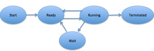
When a process executes, it passes through different states. These stages may differ in different operating systems, and the names of these states are also not standardized.

In general, a process can have one of the following five states at a time.S.N.State & Description1

Start

This is the initial state when a process is first started/created.2

Ready

The process is waiting to be assigned to a processor. Ready processes are waiting to have the processor allocated to them by the operating system so that they can run. Process may come into this state after Start state or while running it by but interrupted by the scheduler to assign CPU to some other process.3

Running

Once the process has been assigned to a processor by the OS scheduler, the process state is set to running and the processor executes its instructions.4

Waiting

Process moves into the waiting state if it needs to wait for a resource, such as waiting for user input, or waiting for a file to become available.5

Terminated or Exit

Once the process finishes its execution, or it is terminated by the operating system, it is moved to the terminated state where it waits to be removed from main memory.

Process Control Block (PCB)

A Process Control Block is a data structure maintained by the Operating System for every process. The PCB is identified by an integer process ID (PID). A PCB keeps all the information needed to keep track of a process as listed below in the table −S.N.Information & Description1

Process State

The current state of the process i.e., whether it is ready, running, waiting, or whatever.2

Process privileges

This is required to allow/disallow access to system resources.3

Process ID

Unique identification for each of the process in the operating system.4

Pointer

A pointer to parent process.5

Program Counter

Program Counter is a pointer to the address of the next instruction to be executed for this process.6

CPU registers

Various CPU registers where process need to be stored for execution for running state.7

CPU Scheduling Information

Process priority and other scheduling information which is required to schedule the process.8

Memory management information

This includes the information of page table, memory limits, Segment table depending on memory used by the operating system.9

Accounting information

This includes the amount of CPU used for process execution, time limits, execution ID etc.10

IO status information

This includes a list of I/O devices allocated to the process.

The architecture of a PCB is completely dependent on Operating System and may contain different information in different operating systems. Here is a simplified diagram of a PCB −

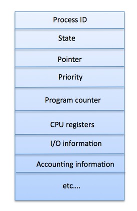
The PCB is maintained for a process throughout its lifetime, and is deleted once the process terminates.

Process Scheduling

Definition

The process scheduling is the activity of the process manager that handles the removal of the running process from the CPU and the selection of another process on the basis of a particular strategy.

Process scheduling is an essential part of a Multiprogramming operating systems. Such operating systems allow more than one process to be loaded into the executable memory at a time and the loaded process shares the CPU using time multiplexing.

Process Scheduling Queues

The OS maintains all PCBs in Process Scheduling Queues. The OS maintains a separate queue for each of the process states and PCBs of all processes in the same execution state are placed in the same queue. When the state of a process is changed, its PCB is unlinked from its current queue and moved to its new state queue.

The Operating System maintains the following important process scheduling queues −

• Job queue − This queue keeps all the processes in the system.
• Ready queue − This queue keeps a set of all processes residing in main memory, ready and waiting to execute. A new process is always put in this queue.
• Device queues − The processes which are blocked due to unavailability of an I/O device constitute this queue.

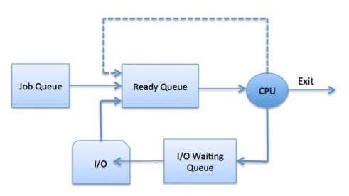
The OS can use different policies to manage each queue (FIFO, Round Robin, Priority, etc.). The OS scheduler determines how to move processes between the ready and run queues which can only have one entry per processor core on the system; in the above diagram, it has been merged with the CPU.

Schedulers

Schedulers are special system software which handle process scheduling in various ways. Their main task is to select the jobs to be submitted into the system and to decide which process to run. Schedulers are of three types −

• Long-Term Scheduler
• Short-Term Scheduler
• Medium-Term Scheduler

Long Term Scheduler

It is also called a job scheduler. A long-term scheduler determines which programs are admitted to the system for processing. It selects processes from the queue and loads them into memory for execution. Process loads into the memory for CPU scheduling.

The primary objective of the job scheduler is to provide a balanced mix of jobs, such as I/O bound and processor bound. It also controls the degree of multiprogramming. If the degree of multiprogramming is stable, then the average rate of process creation must be equal to the average departure rate of processes leaving the system.

On some systems, the long-term scheduler may not be available or minimal. Time-sharing operating systems have no long term scheduler. When a process changes the state from new to ready, then there is use of long-term scheduler.

Short Term Scheduler

It is also called as CPU scheduler. Its main objective is to increase system performance in accordance with the chosen set of criteria. It is the change of ready state to running state of the process. CPU scheduler selects a process among the processes that are ready to execute and allocates CPU to one of them.

Short-term schedulers, also known as dispatchers, make the decision of which process to execute next. Short-term schedulers are faster than long-term schedulers.

Medium Term Scheduler

Medium-term scheduling is a part of swapping. It removes the processes from the memory. It reduces the degree of multiprogramming. The medium-term scheduler is in-charge of handling the swapped out-processes.

A running process may become suspended if it makes an I/O request. A suspended processes cannot make any progress towards completion. In this condition, to remove the process from memory and make space for other processes, the suspended process is moved to the secondary storage. This process is called swapping, and the process is said to be swapped out or rolled out. Swapping may be necessary to improve the process mix.

Operating System Scheduling algorithms

A Process Scheduler schedules different processes to be assigned to the CPU based on particular scheduling algorithms. There are six popular process scheduling algorithms which we are going to discuss in this chapter −

• First-Come, First-Served (FCFS) Scheduling
• Shortest-Job-Next (SJN) Scheduling
• Priority Scheduling
• Shortest Remaining Time
• Round Robin(RR) Scheduling
• Multiple-Level Queues Scheduling

These algorithms are either non-preemptive or preemptive. Non-preemptive algorithms are designed so that once a process enters the running state, it cannot be preempted until it completes its allotted time, whereas the preemptive scheduling is based on priority where a scheduler may preempt a low priority running process anytime when a high priority process enters into a ready state.

First Come First Serve (FCFS)

• Jobs are executed on first come, first serve basis.
• It is a non-preemptive, pre-emptive scheduling algorithm.
• Easy to understand and implement.
• Its implementation is based on FIFO queue.
• Poor in performance as average wait time is high.

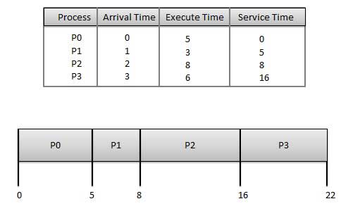
Wait time of each process is as follows −ProcessWait Time : Service Time – Arrival TimeP00 – 0 = 0P15 – 1 = 4P28 – 2 = 6P316 – 3 = 13

Average Wait Time: (0+4+6+13) / 4 = 5.75

Shortest Job Next (SJN)

• This is also known as shortest job first, or SJF
• This is a non-preemptive, pre-emptive scheduling algorithm.
• Best approach to minimize waiting time.
• Easy to implement in Batch systems where required CPU time is known in advance.
• Impossible to implement in interactive systems where required CPU time is not known.
• The processer should know in advance how much time process will take.

Given: Table of processes, and their Arrival time, Execution timeProcessArrival TimeExecution TimeService TimeP0050P1135P22814P3368

Waiting time of each process is as follows −ProcessWaiting TimeP00 – 0 = 0P15 – 1 = 4P214 – 2 = 12P38 – 3 = 5

Average Wait Time: (0 + 4 + 12 + 5)/4 = 21 / 4 = 5.25

Priority Based Scheduling

• Priority scheduling is a non-preemptive algorithm and one of the most common scheduling algorithms in batch systems.
• Each process is assigned a priority. Process with highest priority is to be executed first and so on.
• Processes with same priority are executed on first come first served basis.
• Priority can be decided based on memory requirements, time requirements or any other resource requirement.

Given: Table of processes, and their Arrival time, Execution time, and priority. Here we are considering 1 is the lowest priority.ProcessArrival TimeExecution TimePriorityService TimeP00510P113211P228114P33635

Waiting time of each process is as follows −ProcessWaiting TimeP00 – 0 = 0P111 – 1 = 10P214 – 2 = 12P35 – 3 = 2

Average Wait Time: (0 + 10 + 12 + 2)/4 = 24 / 4 = 6

Shortest Remaining Time

• Shortest remaining time (SRT) is the preemptive version of the SJN algorithm.
• The processor is allocated to the job closest to completion but it can be preempted by a newer ready job with shorter time to completion.
• Impossible to implement in interactive systems where required CPU time is not known.
• It is often used in batch environments where short jobs need to give preference.

Round Robin Scheduling

• Round Robin is the preemptive process scheduling algorithm.
• Each process is provided a fix time to execute, it is called a quantum.
• Once a process is executed for a given time period, it is preempted and other process executes for a given time period.
• Context switching is used to save states of preempted processes.

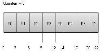
Wait time of each process is as follows −ProcessWait Time : Service Time – Arrival TimeP0(0 – 0) + (12 – 3) = 9P1(3 – 1) = 2P2(6 – 2) + (14 – 9) + (20 – 17) = 12P3(9 – 3) + (17 – 12) = 11

Average Wait Time: (9+2+12+11) / 4 = 8.5

Introduction of Process Synchronization

On the basis of synchronization, processes are categorized as one of the following two types:

• Independent Process : Execution of one process does not affects the execution of other processes.
• Cooperative Process : Execution of one process affects the execution of other processes.

Process synchronization problem arises in the case of Cooperative process also because resources are shared in Cooperative processes.
 
Race Condition
When more than one processes are executing the same code or accessing the same memory or any shared variable in that condition there is a possibility that the output or the value of the shared variable is wrong so for that all the processes doing race to say that my output is correct this condition known as
race condition.
Several processes access and process the manipulations over the same data concurrently, then the outcome depends on the particular order in which the access takes place.
 
Critical Section Problem

Critical section is a code segment that can be accessed by only one process at a time. Critical section contains shared variables which need to be synchronized to maintain consistency of data variables.

In the entry section, the process requests for entry in the Critical Section.

Semaphores

A Semaphore is an integer variable, which can be accessed only through two operations wait() and signal().
There are two types of semaphores : Binary Semaphores and Counting Semaphores

• Binary Semaphores : They can only be either 0 or 1. They are also known as mutex locks, as the locks can provide mutual exclusion. All the processes can share the same mutex semaphore that is initialized to 1. Then, a process has to wait until the lock becomes 0. Then, the process can make the mutex semaphore 1 and start its critical section. When it completes its critical section, it can reset the value of mutex semaphore to 0 and some other process can enter its critical section.
• Counting Semaphores: They can have any value and are not restricted over a certain domain. They can be used to control access to a resource that has a limitation on the number of simultaneous accesses. The semaphore can be initialized to the number of instances of the resource. Whenever a process wants to use that resource, it checks if the number of remaining instances is more than zero, i.e., the process has an instance available. Then, the process can enter its critical section thereby decreasing the value of the counting semaphore by 1. After the process is over with the use of the instance of the resource, it can leave the critical section thereby adding 1 to the number of available instances of the resource.

Classical problems of Synchronization with Semaphore Solution

In this article, we will see number of classical problems of synchronization as examples of a large class of concurrency-control problems. In our solutions to the problems, we use semarphores for synchronization, since that is the traditional way to present such solutions. However, actual implementations of these solutions could use mutex locks in place of binary semaphores.

These problems are used for testing nearly every newly proposed synchronization scheme. The following problems of synchronization are considered as classical problems:

1. Bounded-buffer (or Producer-Consumer) Problem,
2. Dining-Philosphers Problem,
3. Readers and Writers Problem,
4. Sleeping Barber Problem

These are summarized, for detailed explanation, you can view the linked articles for each.

1. :Producer consumer problem
   Bounded Buffer problem is also called producer consumer problem. This problem is generalized in terms of the Producer-Consumer problem. Solution to this problem is, creating two counting semaphores “full” and “empty” to keep track of the current number of full and empty buffers respectively. Producers produce a product and consumers consume the product, but both use of one of the containers each time.
   1. Dining philosopher problem:
      The Dining Philosopher Problem states that K philosophers seated around a circular table with one chopstick between each pair of philosophers. There is one chopstick between each philosopher. A philosopher may eat if he can pickup the two chopsticks adjacent to him. One chopstick may be picked up by any one of its adjacent followers but not both. This problem involves the allocation of limited resources to a group of processes in a deadlock-free and starvation-free manner.<img class=”i-amphtml-intrinsic-sizer” alt=”” src=”data:image/svg+xml;charset=utf-8,” />

1. Readers and writers problem:
   Suppose that a database is to be shared among several concurrent processes. Some of these processes may want only to read the database, whereas others may want to update (that is, to read and write) the database. We distinguish between these two types of processes by referring to the former as readers and to the latter as writers. Precisely in OS we call this situation as the readers-writers problem. Problem parameters:
   • One set of data is shared among a number of processes.
   • Once a writer is ready, it performs its write. Only one writer may write at a time.
   • If a process is writing, no other process can read it.
   • If at least one reader is reading, no other process can write.
   • Readers may not write and only read.
2. Sleeping Barber Problem:
   Barber shop with one barber, one barber chair and N chairs to wait in. When no customers the barber goes to sleep in barber chair and must be woken when a customer comes in. When barber is cutting hair new custmers take empty seats to wait, or leave if no vacancy.