Device management in operating system known as the management of the I/O devices such as a keyboard, magnetic tape, disk, printer, microphone, USB ports, scanner, etc.as well as the supporting units like control channels.

Technique of device management in the operating system

An operating system or the OS manages communication with the devices through their respective drivers. The operating system component provides a uniform interface to access devices of varied physical attributes. For device management in operating system:

• Keep tracks of all devices and the program which is responsible to perform this is called I/O controller.
• Monitoring the status of each device such as storage drivers, printers and other peripheral devices.
• Enforcing preset policies and taking a decision which process gets the device when and for how long.
• Allocates and Deallocates the device in an efficient way.De-allocating them at two levels: at the process level when I/O command has been executed and the device is temporarily released, and at the job level, when the job is finished and the device is permanently released.
• Optimizes the performance of individual devices.

Types of devices

The OS peripheral devices can be categorized into 3: Dedicated, Shared, and Virtual. The differences among them are the functions of the characteristics of the devices as well as how they are managed by the Device Manager.

Dedicated devices:-

Such type of devices in the device management in operating system are dedicated or assigned to only one job at a time until that job releases them. Devices like printers, tape drivers, plotters etc. demand such allocation scheme since it would be awkward if several users share them at the same point of time. The disadvantages of such kind f devices s the inefficiency resulting from the allocation of the device to a single user for the entire duration of job execution even though the device is not put to use 100% of the time.

Shared devices:-

These devices can be allocated o several processes. Disk-DASD can be shared among several processes at the same time by interleaving their requests. The interleaving is carefully controlled by the Device Manager and all issues must be resolved on the basis of predetermined policies.

Virtual Devices:-

These devices are the combination of the first two types and they are dedicated devices which are transformed into shared devices. For example, a printer converted into a shareable device via spooling program which re-routes all the print requests to a disk. A print job is not sent straight to the printer, instead, it goes to the disk(spool)until it is fully prepared with all the necessary sequences and formatting, then it goes to the printers. This technique can transform one printer into several virtual printers which leads to better performance and use.

input/output devices

input/Output devices are the devices that are responsible for the input/output operations in a computer system.

Basically there are following two types of input/output devices:

• Block devices
• Character devices

Block Devices

A block device stores information in block with fixed-size and own-address.

It is possible to read/write each and every block independently in case of block device.

In case of disk, it is always possible to seek another cylinder and then wait for required block to rotate under head without mattering where the arm currently is. Therefore, disk is a block addressable device.

Character Devices

A character device accepts/delivers a stream of characters without regarding to any block structure.

Character device isn’t addressable.

Character device doesn’t have any seek operation.

There are too many character devices present in a computer system such as printer, mice, rats, network interfaces etc. These four are the common character devices.

Input/Output Devices Examples

Here are the list of some most popular and common input/output devices:

• Keyboard
• Mouse
• Monitor
• Modem
• Scanner
• Laser Printer
• Ethernet
• Disk

Storage devices

There are two types of storage devices:-

• Volatile Storage Device –
  It looses its contents when the power of the device is removed.
• Non-Volatile Storage device –
  It does not looses its contents when the power is removed. It holds all the data when the power is removed.

Secondary Storage is used as an extension of main memory. Secondary storage devices can hold the data permanently.
Storage devices consists of Registers, Cache, Main-Memory, Electronic-Disk, Magnetic-Disk, Optical-Disk, Magnetic-Tapes. Each storage system provides the basic system of storing a datum and of holding the datum until it is retrieved at a later time. All the storage devices differ in speed, cost, size and volatility. The most common Secondary-storage device is a Magnetic-disk, which provides storage for both programs and data.

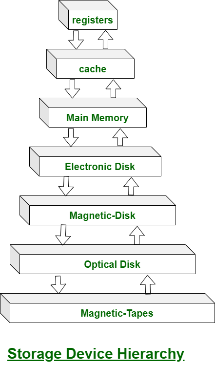
In this hierarchy all the storage devices are arranged according to speed and cost. The higher levels are expensive, but they are fast. As we move down the hierarchy, the cost per bit generally decreases, where as the access time generally increases.

The storage systems above the Electronic disk are Volatile, where as those below are Non-Volatile.
An Electronic disk can be either designed to be either Volatile or Non-Volatile. During normal operation, the electronic disk stores data in a large DRAM array, which is Volatile. But many electronic disk devices contain a hidden magnetic hard disk and a battery for backup power. If external power is interrupted, the electronic disk controller copies the data from RAM to the magnetic disk. When external power is restored, the controller copies the data back into the RAM.

The design of a complete memory system must balance all the factors. It must use only as much expensive memory as necessary while providing as much inexpensive, Non-Volatile memory as possible. Caches can be installed to improve performance where a large access-time or transfer-rate disparity exists between two components.

Buffering

A buffer is a memory area that stores data being transferred between two devices or between a device and an application.

Uses of I/O Buffering :

• Buffering is done to deal effectively with a speed mismatch between the producer and consumer of the data stream.
• A buffer is produced in main memory to heap up the bytes received from modem.
• After receiving the data in the buffer, the data get transferred to disk from buffer in a single operation.
• This process of data transfer is not instantaneous, therefore the modem needs another buffer in order to store additional incoming data.
• When the first buffer got filled, then it is requested to transfer the data to disk.
• The modem then starts filling the additional incoming data in the second buffer while the data in the first buffer getting transferred to disk.
• When both the buffers completed their tasks, then the modem switches back to the first buffer while the data from the second buffer get transferred to the disk.
• The use of two buffers disintegrates the producer and the consumer of the data, thus minimizes the time requirements between them.
• Buffering also provides variations for devices that have different data transfer sizes.

Types of various I/O buffering techniques :

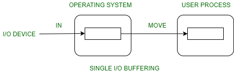
1. Single buffer :
A buffer is provided by the operating system to the system portion of the main memory.

Block oriented device –

• System buffer takes the input.
• After taking the input, the block gets transferred to the user space by the process and then the process requests for another block.
• Two blocks works simultaneously, when one block of data is processed by the user process, the next block is being read in.
• OS can swap the processes.
• OS can record the data of system buffer to user processes.

Stream oriented device –

• Line- at a time operation is used for scroll made terminals. User inputs one line at a time, with a carriage return signaling at the end of a line.
• Byte-at a time operation is used on forms mode, terminals when each keystroke is significant.

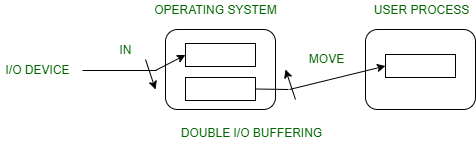
2. Double buffer :

Block oriented –

• There are two buffers in the system.
• One buffer is used by the driver or controller to store data while waiting for it to be taken by higher level of the hierarchy.
• Other buffer is used to store data from the lower level module.
• Double buffering is also known as buffer swapping.
• A major disadvantage of double buffering is that the complexity of the process get increased.
• If the process performs rapid bursts of I/O, then using double buffering may be deficient.

Stream oriented –

• Line- at a time I/O, the user process need not be suspended for input or output, unless process runs ahead of the double buffer.
• Byte- at a time operations, double buffer offers no advantage over a single buffer of twice the length.

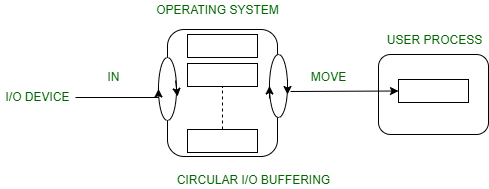
3. Circular buffer :

• When more than two buffers are used, the collection of buffers is itself referred to as a circular buffer.
• In this, the data do not directly passed from the producer to the consumer because the data would change due to overwriting of buffers before they had been consumed.
• The producer can only fill up to buffer i-1 while data in buffer i is waiting to be consumed.

Secondry storage structure

Secondary storage devices are those devices whose memory is non volatile, meaning, the stored data will be intact even if the system is turned off. Here are a few things worth noting about secondary storage.

• Secondary storage is also called auxiliary storage.
• Secondary storage is less expensive when compared to primary memory like RAMs.
• The speed of the secondary storage is also lesser than that of primary storage.
• Hence, the data which is less frequently accessed is kept in the secondary storage.
• A few examples are magnetic disks, magnetic tapes, removable thumb drives etc.

---

Magnetic Disk Structure

In modern computers, most of the secondary storage is in the form of magnetic disks. Hence, knowing the structure of a magnetic disk is necessary to understand how the data in the disk is accessed by the computer.

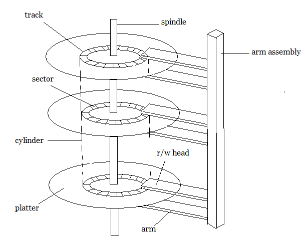
Structure of a magnetic disk

A magnetic disk contains several platters. Each platter is divided into circular shaped tracks. The length of the tracks near the centre is less than the length of the tracks farther from the centre. Each track is further divided into sectors, as shown in the figure.

Tracks of the same distance from centre form a cylinder. A read-write head is used to read data from a sector of the magnetic disk.

The speed of the disk is measured as two parts:

• Transfer rate: This is the rate at which the data moves from disk to the computer.
• Random access time: It is the sum of the seek time and rotational latency.

Seek time is the time taken by the arm to move to the required track. Rotational latency is defined as the time taken by the arm to reach the required sector in the track.

Even though the disk is arranged as sectors and tracks physically, the data is logically arranged and addressed as an array of blocks of fixed size. The size of a block can be 512 or 1024 bytes. Each logical block is mapped with a sector on the disk, sequentially. In this way, each sector in the disk will have a logical address.

---

Disk Scheduling Algorithms

On a typical multiprogramming system, there will usually be multiple disk access requests at any point of time. So those requests must be scheduled to achieve good efficiency. Disk scheduling is similar to process scheduling. Some of the disk scheduling algorithms are described below.

---

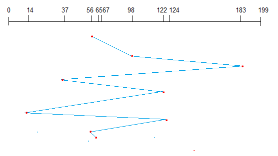
First Come First Serve

This algorithm performs requests in the same order asked by the system. Let’s take an example where the queue has the following requests with cylinder numbers as follows:

98, 183, 37, 122, 14, 124, 65, 67

Assume the head is initially at cylinder 56. The head moves in the given order in the queue i.e., 56→98→183→…→67.

---

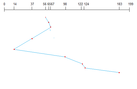
Shortest Seek Time First (SSTF)

Here the position which is closest to the current head position is chosen first. Consider the previous example where disk queue looks like,

98, 183, 37, 122, 14, 124, 65, 67

Assume the head is initially at cylinder 56. The next closest cylinder to 56 is 65, and then the next nearest one is 67, then 37, 14, so on.

---

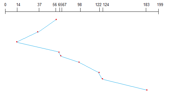
SCAN algorithm

This algorithm is also called the elevator algorithm because of it’s behavior. Here, first the head moves in a direction (say backward) and covers all the requests in the path. Then it moves in the opposite direction and covers the remaining requests in the path. This behavior is similar to that of an elevator. Let’s take the previous example,

98, 183, 37, 122, 14, 124, 65, 67

Assume the head is initially at cylinder 56. The head moves in backward direction and accesses 37 and 14. Then it goes in the opposite direction and accesses the cylinders as they come in the path.

Disk management

The operating system is responsible for several aspects of disk management.

Disk Formatting

A new magnetic disk is a blank slate. It is just platters of a magnetic recording material. Before a disk can store data, it must be divided into sectors that the disk controller can read and write. This process is called low-level formatting (or physical formatting).

Low-level formatting fills the disk with a special data structure for each sector. The data structure for a sector consists of a header, a data area, and a trailer. The header and trailer contain information used by the disk controller, such as a sector number and an error-correcting code (ECC).

To use a disk to hold files, the operating system still needs to record its own data structures on the disk. It does so in two steps. The first step is to partition the disk into one or more groups of cylinders. The operating system can treat each partition as though it were a separate disk. For instance, one partition can hold a copy of the operating system’s executable code, while another holds user files. After partitioning, the second step is logical formatting (or creation of a file system). In this step, the operating system stores the initial file-system data structures onto the disk.

Boot block

When a computer is powered up or rebooted, it needs to have an initial program to run. This initial program is called the bootstrap program. It initializes all aspects of the system (i.e. from CPU registers to device controllers and the contents of main memory) and then starts the operating system.

To do its job, the bootstrap program finds the operating system kernel on disk, loads that kernel into memory, and jumps to an initial address to begin the operating-system execution.

For most computers, the bootstrap is stored in read-only memory (ROM). This location is convenient because ROM needs no initialization and is at a fixed location that the processor can start executing when powered up or reset. And since ROM is read-only, it cannot be infected by a computer virus. The problem is that changing this bootstrap code requires changing the ROM hardware chips.

For this reason, most systems store a tiny bootstrap loader program in the boot ROM, whose only job is to bring in a full bootstrap program from disk. The full bootstrap program can be changed easily: A new version is simply written onto the disk. The full bootstrap program is stored in a partition (at a fixed location on the disk) is called the boot blocks. A disk that has a boot partition is called a boot disk or system disk.

Bad Blocks

Since disks have moving parts and small tolerances, they are prone to failure. Sometimes the failure is complete, and the disk needs to be replaced, and its contents restored from backup media to the new disk.

More frequently, one or more sectors become defective. Most disks even come from the factory with bad blocks. Depending on the disk and controller in use, these blocks are handled in a variety of ways.

The controller maintains a list of bad blocks on the disk. The list is initialized during the low-level format at the factory and is updated over the life of the disk. The controller can be told to replace each bad sector logically with one of the spare sectors. This scheme is known as sector sparing or forwarding.

Swap-space management

Swapping is a memory management technique used in multi-programming to increase the number of process sharing the CPU. It is a technique of removing a process from main memory and storing it into secondary memory, and then bringing it back into main memory for continued execution. This action of moving a process out from main memory to secondary memory is called Swap Out and the action of moving a process out from secondary memory to main memory is called Swap In.

Swap-Space :
The area on the disk where the swapped out processes are stored is called swap space.

Swap-Space Management :
Swap-Swap management is another low-level task pf the operating system. Disk space is used as an extension of main memory by the virtual memory. As we know the fact that disk access is much slower than memory access, In the swap-space management we are using disk space, so it will significantly decreases system performance. Basically, in all our systems we require the best throughput, so the goal of this swap-space implementation is to provide the virtual memory the best throughput.

 Swap-Space Use :
Swap-space is used by the different operating-system in various ways. The systems which are implementing swapping may use swap space to hold the entire process which may include image, code and data segments. Paging systems may simply store pages that have been pushed out of the main memory. The need of swap space on a system can vary from a megabytes to gigabytes but it also depends on the amount of physical memory, the virtual memory it is backing and the way in which it is using the virtual memory.

A swap space can reside in one of the two places –

1. Normal file system
2. Separate disk partition

Let, if the swap-space is simply a large file within the file system. To create it, name it and allocate its space normal file-system routines can be used. This approach, through easy to implement, is inefficient. Navigating the directory structures and the disk-allocation data structures takes time and extra disk access. During reading or writing of a process image, external fragmentation can greatly increase swapping times by forcing multiple seeks.

There is also an alternate to create the swap space which is in a separate raw partition. There is no presence of any file system in this place. Rather, a swap space storage manager is used to allocate and de-allocate the blocks. from the raw partition. It uses the algorithms for speed rather than storage efficiency, because we know the access time of swap space is shorter than the file system. By this Internal fragmentation increases, but it is acceptable, because the life span of the swap space is shorter than the files in the file system. Raw partition approach creates fixed amount of swap space in case of the disk partitioning.

Some operating systems are flexible and can swap both in raw partitions and in the file system space, example: Linux.

Disk reliability